Query2 and differential dataflow

Along with timely-dataflow, Frank McSherry develops and maintains another library focusing on efficient data processing: differential-dataflow. This week, we’ll have a look at what it brings to the table.

Introducing differential dataflow

The previous post gave us an insight of what kind of development work is involved in translating relational operators to a timely-dataflow implementation. Let’s just say it has a distinct taste of pre-pig-pre-hive-pre-spark-all-by-hand Hadoop MapReduce. But that’s fine. It’s what it’s meant to be. Low-level routines for higher-level libraries.

Differential dataflow is one of these more specialized and higher level library. At its core, it proposes a radical approach to the “lambda architecture” problem. The idea of lambda architecture is to build data systems that provide seamlessly real-time dashboards and historical data. People have managed this by either combining two different systems, or choosing one and hammering it until it fits in the other hole.

Differential dataflow does it by defining streams of data as incremental differences to be integrated in a “live” result. Typically, every record of data in a stream is associated with a weight: +1 for addition, -1 for removal.

On top of this streaming protocol, differential dataflown goes the extra mile to provide difference-aware relational operators. The ones we know and have learn to expect. map, group, join. No more need to get into map/reduce witchery.

And if we just consider our dataset as one big stream of differences from an empty state, ingesting every record with a +1 weight should get us to the result, right ? We’ll try that.

Query 2 in differential dataflow

If you’re joining us here, let’s briefly recap the exercice: we try to perform the following aggregation query using various technologies in the nascent rust ecosystem.

  SELECT SUBSTR(sourceIP, 1, 8), SUM(adRevenue)
    FROM uservisits
GROUP BY SUBSTR(sourceIP, 1, 8)

We will compute the full result in memory, because it fits, but merely display the count of records to check what we have done.

So this week, we will play with differential dataflow.

The code is here. Timely version was here.

You may want to refer to the timely version commentary in the previous post.

The code first defines a SaneF32 (this is us just f32 wrapper to define Ord and Hash on f32, because I know there are no NaN in the data), which is not directly relevant for us. TL;DR ? SaneF32 is a single precision float, just like rust f32, that we will be using for ad_revenue.

Then comes a main function, yielding to timely::execute_from_args to manage distribution and worker instantiation.

Each worker starts with picking the right subset of files it is responsible to deal with as input to the global system then defines the dataflow graph.

First, I’d like to comment on what is actually pushed in the graph, in the very last lines.

for visit in uservisits {
    let key = Bytes8::prefix(&*visit.0);
    let value = SaneF32(visit.1);
    let weight = 1;
    input.send( ((key, value), weight) );
}

This is a pair of a datum and a weight (+1), the datum itself is made of a key (an instance of Bytes8) and a value (the sane f32). input.send() adds the timely timestamp behind the scene, and we are pushing everything in one big batch.

The graph itself is defined in the root::scoped call. The handle it returns is the input we have just used to push data into the graph. This input is itself created inside the scope in the first of the following two lines:

let (input, stream) = builder.new_input::<((Bytes8, SaneF32), i32)>();
let collection = Collection::new(stream);

Collection is the differential dataflow struct that supports the differential protocol. It wraps our input stream.

let group: Collection<_, (Bytes8, SaneF32)> = 
    collections.group(|_key, values, output| {
        let v: f32 = values
            .map(|(sane, weight): (&SaneF32, i32)| 
                sane.0 * weight as f32)
            .sum();
        output.push((SaneF32(v), 1));
    });

Then we implement the Query2 groupby with a single group call on collection. It expects the datum to be in a (K,V) form, and gives the caller a chance to specify how the values for a given key should be aggregated. This aggregator is a closure in our case. It will be called once or more times for each different key, and will be passed the key itself, a list of values to aggregate, and an output handler to push the result to.

This aggregator has to take into account the weight: we are dealing in differences here. So the values iterator does not contain raw values, but pairs of value and weight (+1 or -1).

If a visit disappear from the input, its weight would be -1, and it revenue should be subtracted from the final result: multiplying the value by the weight will just do the right thing.

Of course, our input only adds stuff: all records have a weight of +1 so this is basically cosmetic. Once we have summed these differences, we push the result, with a weight of +1 to our output (using again then sane f32 wrapper).

The group() method return a Collection handle that will let us chain other operators on our stream of data. In our case, after the group operator from the pseudo-sql query, we plug in the count operator that we use to check the result:

let count: Collection<_, (bool, u32)> =
    group.map(|(_, _): (Bytes8, SaneF32)| { (true, 1) });

let count: Collection<_, (bool, i32)> = count.group(|_, values, output| {
    let count: i32 = values
        .map(|(count, weight): (&u32, i32)| *count as i32 * weight)
        .sum();
    output.push((count, 1));
});

Differential dataflow does not have a built-in count(), but as we have seen in the previous post, a count can be implemented by mapping records to a single key with a value of 1, and summing these 1s values. I use true as the magical single key, and perform the partial sum of the 1s values in a very similar fashion than in the group operation, multiplying whatever I wanted added by the weight — probably always +1— then push the result with a weight of — you guessed it — +1.

count.inspect(move |record| println!("XXX {} XXX", (record.0).1));

Finally, we display the result, or at least the relevant part of it: it is buried in two nested tuples: the full record is actually ( (true, result), weight) where true is the magic aggregation key we picked before, and weight is… +1.

The code feels kind of “right” in term of volume of boilerplate. It could still be a bit more compact, it would be nice to have a built-on count() operator, but lots of boilerplate from the timely implementation has gone away. On the other hand, having to deal with the weight adds some cognitive cost to what we are actually trying to achieve.

Results

Does it works ? Yes. I do get the correct result. Is it efficient ? Mmm no. Not that much. At least not on the laptop. Nearly 200 seconds.

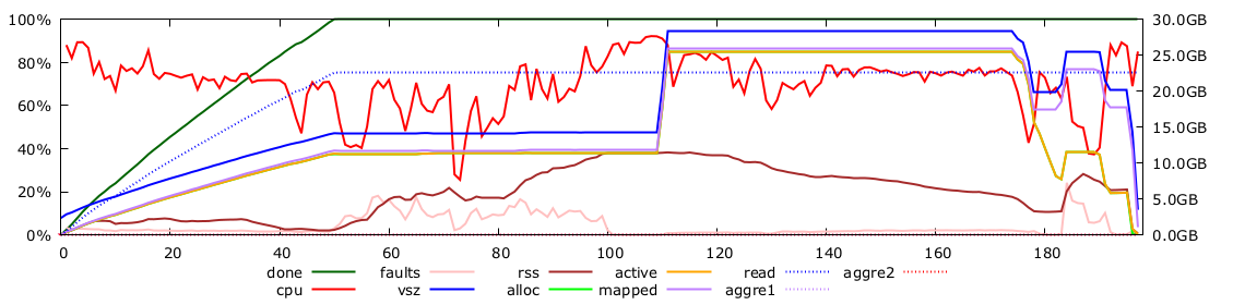
Remember timely dataflow performance ? Below 50 seconds on my laptop.

Aside the cognitive cost, there is an actual technical cost to considering the data incrementally: lots of stuff has to stay around in memory. In the general case, differential dataflow needs to keep stuff alive to be able to perform the right aggregation in the data: for instance, a record with an ad_revenue of zero could either be an added and removed results (which should not appear in the result final) or just the result of a unlikely sum of ad_revenue that make zero (given that they are positive, very unlikely, but differential dataflow operartors can not know about that).

In the timely dataflow implementation, all that we have to keep in memory is the result HashMap. We have discussed at length how we could make it fit in less ~10GB even for the demanding 2C case. 2A in timely needs about 300MB of memory. In differential it activates about 25GB, so it swaps a lot and gets slow.

I was expecting some cost, I did not think it would be so high.

Differential dataflow

Bottom line is, differential dataflow focuses on a different problem than the one I was trying to optimize. It manages it, correctly, but not as efficiently as timely dataflow does.

Let’s give it a chance to shine though, because it is interesting. Lambda architecture issue is interesting. Let’s imagine we have a website running with a ton of historical data, and want to get the aggregation result of Query2 in real time. Just pretend.

The input is made of 2037 input files. We will consider the first 95% files as historical data, and then dribble the remaining ones as incremental updates.

Setting this up takes a bit of work, the API is a bit tricky, probably not fully sorted out yet. We need a way to know the graph has digested everything it has ingested before moving to the next chunk. It requires to use something called a “probe”. I won’t get into the details, the code is around here if you fell compelled to.

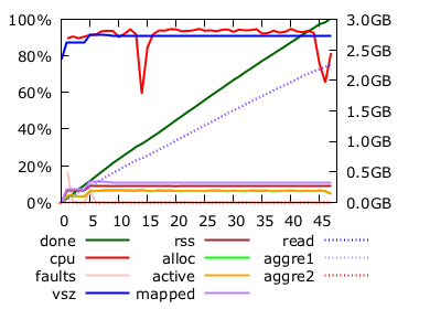
We’ll just go and get a big instance on EC2 to get the memory consumption issue out of the way. I picked the c3.8xlarge monster.

43.453s:  stepped over initial batch result:2060191
45.612s:  done step 1, results: 2060611
48.005s:  done step 2, results: 2061043
50.486s:  done step 3, results: 2061519
52.713s:  done step 4, results: 2061918
54.538s:  done step 5, results: 2062337
56.322s:  done step 6, results: 2062749
58.130s:  done step 7, results: 2063181
59.960s:  done step 8, results: 2063572
61.845s:  done step 9, results: 2063964
64.356s:  done step 10, results: 2064354
66.336s:  done step 11, results: 2064740
68.446s:  done step 12, results: 2065140
70.510s:  done step 13, results: 2065521
72.804s:  done step 14, results: 2065929
75.264s:  done step 15, results: 2066283
77.416s:  done step 16, results: 2066642
79.692s:  done step 17, results: 2067050
81.823s:  done step 18, results: 2067317

And here we go. After about 43 seconds for processing the “historical” dataset, we perform integration of the real-time data chunks in roughly 2 seconds each. In batch mode with timely-dataflow with the full dataset, the best time I managed to get with this configuration was 16 seconds. So here, differential dataflow brings a way to integrate results for real time in a fraction (about 1/8) of the time it would need to reprocess the full data.

Of course, depending on the size of the historical data versus the increment size, leaving the brutal efficiency of timely dataflow in favor of the more demanding differential dataflow may or may not make sense.

Frank McSherry has blogged extensively on how this still works with algorithms requiring iterations — BFS for instance. It’s quite impressive.

Conclusion

We learn something more here. Differential dataflow API gives us a glimpse at what a “relational oriented” API may look like if someone would try to go for it: relational operators from differential, implemented over timely, without the differential part of it.

I don’t know for you, but I kind of like what it looks like.

Rust and BigData series:

1. Rust, BigData and my laptop
2. The rust is in there
3. Let’s optimize
4. Hashes to hashes
5. Embrace the glow cloud
6. Query2 in timely dataflow
7. Query2 in differential dataflow