
Embrace the glow cloud
15 Feb 2016This is part #5 of a series about a BigData in Rust experiment.
We are working on a simple query nicknamed Query2 and comparing our results to the BigData benchmark.
  SELECT SUBSTR(sourceIP, 1, X), SUM(adRevenue)
    FROM uservisits
GROUP BY SUBSTR(sourceIP, 1, X)
| Query | X | group count | Hive | Shark | Redshift | My laptop |
|---|---|---|---|---|---|---|
| 2A | 8 | 2,067,313 | 730s | 83s | 25s | 50s |
| 2B | 10 | 31,348,913 | 764s | 100s | 56s | 64s |
| 2C | 12 | 253,890,330 | 730s | 132s | 79s | 91s |
The last column is what we manage to get on my laptop using Rust, with quite a lot of work and trying to stay in the realm of “fair” optimisations that an automatic query planner could find.
The other columns are partial results from the BigData benchmark, running on a 8$/hr on Amazon EC2.
So let’s do the same. Let’s go to EC2 and buy us a 8$/hr cluster.
Timely dataflow
My implementation of Query2 is not distributable. It is multithreaded, but can not span processes or hosts. Doing this by hand would be a lot of work, but the Rust ecosystem provides a little gem called Timely dataflow.
Timely dataflow is designed as a low-level toolbox for distributing work. To quote the README, it is a “low-latency cyclic dataflow computational model”. Frank McSherry experimented with the concept of timely dataflow while working on Naiad at Microsoft Research, and has since ported it from C# to Rust.
Integrating Query2 in timely has not been very difficult — even if I had to get some help from higher deities — but induced a change in the general algorithm which I have described in the previous post.
It turns out the way timely lead me to write the aggregation is about 10% more efficient than my ad-hoc implementation, so I won’t complain. I have not completely explored the reason that make it so. Re-organising the ad-hoc implementation so that the data flows in a way similar to the way it flows in the timely program may help.
Anyway. Let’s go to the ec2 pricing page. The sky is the limit, up to 8$/hr.
Tweaking an EC2 cluster
EBS disks tends to make things less predictable, so we will start with instances having enough SSD as local storage. We want to try “work-horse” instances (m series) but as we have established we need to care about CPU, we also want to try instances from the C series.
So eligible are m3 and c3. m3.medium and m3.large have not enough disk space, leaving us with m3.xlarge and m3.2xlarge, at a cost of $0.266 and $0.532 per hour respectively.
The c3 series is more plentiful in terms of choice: c3.large would barely contains our data, but c3.xlarge, c3.2xlarge, c3.4xlarge or even the huge c3.8xlarge (36 cores, 60GB) are eligible. We could still afford 5 of these things with our $8 budget.
To make things more interesting, my early tries and conversations with the timely dataflow team lead to the realisation that there was a particular parameter that had a huge impact on the performance of a timely cluster. This parameter is the worker number. More about that in a minute.
The cheapest possible M choice is m3.xlarge. This instance is $0.266 per Hour, so we would need 30 of them to get to get to the 8$/hr mark.
And of course, we have the three query variants (A, B, C).
All in all, this leaves me with a huge multi-dimensional space to explore. I’m not sure it contains much in terms of black holes chirping, but it’s big. And as much as I don’t care much about using my laptop as a (noisy) heater in these cold times, I’m not too keen in spending too much on EC2 on my own. Bottom line is, I can’t offer you an exhaustive exploration. Let’s just say I have found a few sweet spots.
Sweet spots
First, let’s try a cluster made of the biggest instance possible, c3.8xlarge. It has 36 cores, two SSD drives that are only marginally better than ones available on other instances (the stripped raid setup provides about 1GB/s). Spoiler: in standalone mode, this instance actually manages to saturate the SSD bandwidth.
For $8/hr, we can afford five of them.
| Query | X | group count | Hive | Shark | Redshift | My laptop | 5 * c3.8xlarge |
|---|---|---|---|---|---|---|---|
| 2A | 8 | 2,067,313 | 730s | 83s | 25s | 50s | 4.7s |
| 2B | 10 | 31,348,913 | 764s | 100s | 56s | 64s | 5.9s |
| 2C | 12 | 253,890,330 | 730s | 132s | 79s | 91s | 6.0s |
Now this took some work. I was initially running with a number of workers equals to twice the number of cpus. The timely guys initially suggested I try a figure a bit under the number of cpus. It turns out the best value I could find was around 10 workers, so a small third of the number of cpus…
Well that’s the thing. We are in uncharted territory. From my understanding, Frank’s at-scale experiments with timely are mostly revolving about in-memory graph processing, so our spark-like load might be one of the first to go there (or to report it). Here be baboons!
Nevertheless, five times faster than Redshift for the same cost is not so bad, right ?
For a smaller price, we can pool more instances at a lesser cost and get very decent performance:
| Query | Shark | Redshift | 5*c3.8xl | 10*c3.2xl | 10*m3.2xl | 20*m3.xl |
|---|---|---|---|---|---|---|
| cost | $8.20 | $8.50 | $8.40 | $4.20 | $5.32 | $5.32 |
| 2A | 83s | 25s | 4.7s | 6.8s | 6.4s | 6.0s |
| 2B | 100s | 56s | 5.9s | 8.7s | 9.5s | 8.5s |
| 2C | 132s | 79s | 6.0s | 9.1s | 10.1s | 9.8s |
We already have a very positive answer to our initial interrogation: we managed to get roughly five time — in the less favorable case — faster than Redshift for the same price! And comparing to Shark is even more edifying.
Second question: how cost efficient is this? Let’s try to normalize these results a bit and eliminate a few magic numbers. We’ll focus on the bandwidth / $ and use the Redfshift numbers from the BigData benchmark as a reference.
So, the bigger, the better. The higher the figure, the more you’ll get for your money.
| Query | Shark | Redshift | 5*c3.8xl | 10*c3.2xl | 10*m3.2xl | 20*m3.xl |
|---|---|---|---|---|---|---|
| 2A | 0.29 | 1 | 5.3 | 7.4 | 6.2 | 6.7 |
| 2B | 0.54 | 1 | 9.6 | 13.0 | 9.5 | 10.5 |
| 2C | 0.57 | 1 | 13.3 | 17.5 | 12.5 | 12.9 |
Scalability
These configuration were chosen arbitrarily, to try to get some intuition about the all-important worker number, but for all we know, a 10-node m3.xl could perform nearly as well as the 20-node for half the cost. So let’s start exploring this dimension a bit.
The absolute Graal, in scalability, is linear scalability. Linear scalability means you will have your process running twice as fast when you double the amount of resources you allocate to it. It’s the very comfortable zone where, when faced with a 2000hr.core compute, you can get your result using on one single core for 2000 hours, or in one hour by using 2000 cores, at the same cost. In terms of our normalized efficiency measure, ideally, it should not depend on the number of nodes we use.
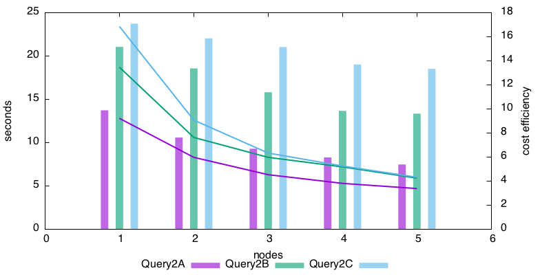
So let’s see how this figures behave when we change the number of hosts. Note that the worker count need to be adjusted on the way. The optimum seems to be at number-of-cores - 1 for small cluster, and down to a fraction of the number-of-cores (around one third) for the bigger cluster configuration I have tried. Intuitively, as the cluster grows, there is more stuff to be exchanged with peers, so the worker thread count (that the parameter control) has to be reduced to leave more space to the background networking thread.
This is for the 5*c3.8xlarge cluster. The lines show the duration of the process, the bars are cost-efficiency comparing to RedShift.
and this is for the 20*m3.xlarge.
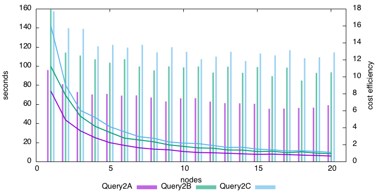
Now what is very nice about the second graph is, the height of the efficiency bars is nearly constant after five nodes. It means we are not very far from the Graal of linear scalability. The c3.xlarge graph is less nice-looking, but we may just be in the initial zone of the graph, where the cost of going distributed is still being amortized. I have not tried testing with more nodes, because 1/ these beasts are not cheap, 2/ accuracy is becoming a factor in the time measure as the running time get shorter and shorter.
Recap
So what can we learn with these experiments on ec2?
- timely dataflow allows us to go distributed with a very reasonable development overhead
- timely implementation is lean. Despite introducing abstraction, the standalone test is better than an ad-hoc implementation — alternative explanation: I’m really bad at this
- despite being young, timely has a very decent efficiency response in this use case.
So there is lot of potential here. Somebody needs to make BigData tools in Rust :)
Rust and BigData series: